The 2018 European heat wave

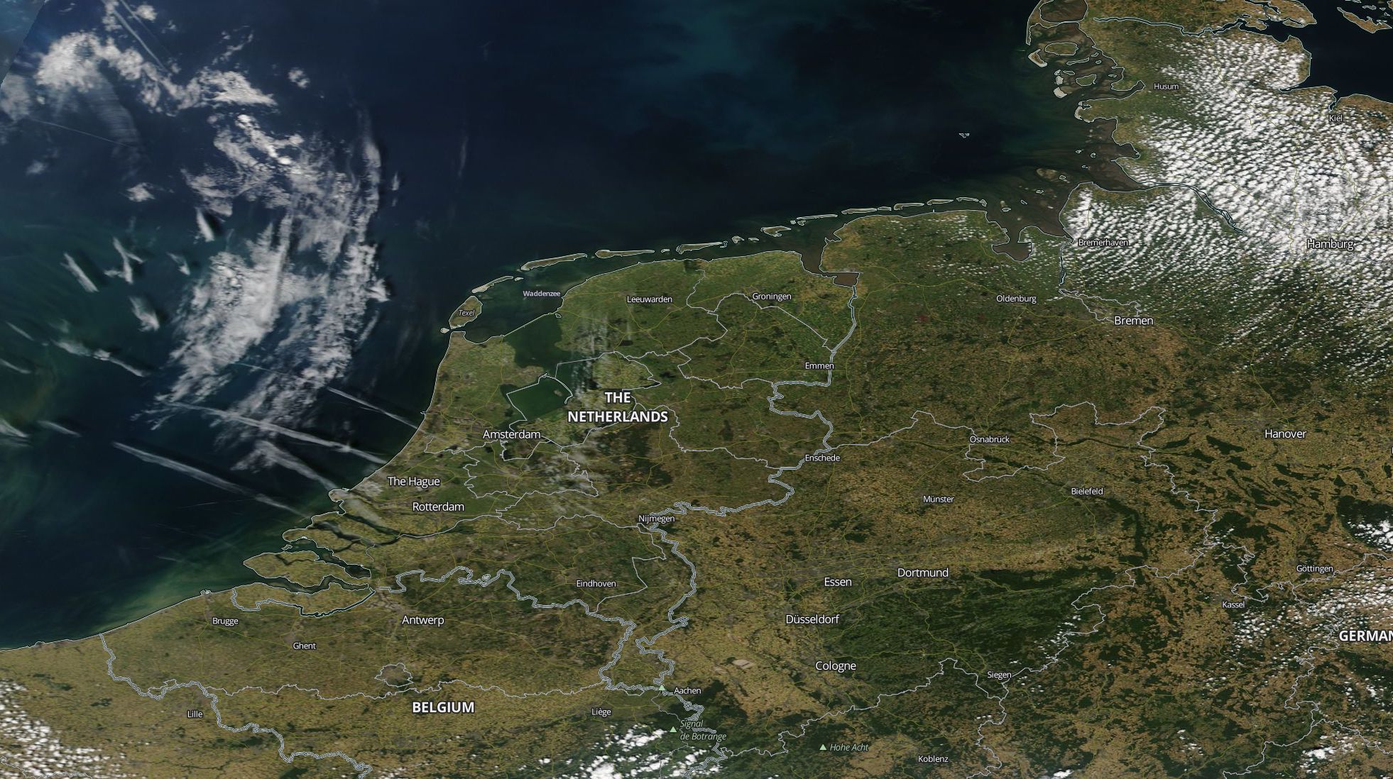
MODIS Corrected Reflectance imagery for the 15 July 2018 (@NASA).

In this example tutorial we show how to use WRF-CMake to simulate 6 hours, for an area centered in Amsterdam, for the 15 July 2018 (12:00 - 18:00) related to the heat wave that affected the Netherlands between the 15 and 27 July 2018. You should be able to complete this tutorial in less than 20 minutes, including simulation. On an average machine, dual core @ 2.4 GHz with 8 GB of RAM, this 6-hour simulation should take no more than 5 minutes to complete.

Software requirements

• WRF-CMake
• Python 3.x

Overview

The whole process from configuration to running the simulation and visualization of outputs will take no more than 20 minutes on an average machine. This process can be broken down in the following 5 main steps:

• The 2018 European heat wave
• Overview
• Download geographical data
• Download meteorological data
• Configure and run WPS
  • Run Geogrid
  • Run Ungrib
  • Run Metgrid
• Configure and run WRF
  • Run Real
  • Run WRF
• View the results

Download geographical data

Download the Lowest Resolution of Each Mandatory Field dataset and decompress them in DATA/geog.

Download meteorological data

In this example we use NCEP GDAS/FNL 0.25 Degree Global Tropospheric Analyses and Forecast Grids as initial and boundary conditions. To download the data, go to https://rda.ucar.edu/datasets/ds083.3 and log-in. From the Data Access tab, click on Get a Subset and fill in your request with the following configuration:

• Dataset: ds083.3
• Product: Analysis
• Variables: all
• Output Format: Same as input
• Start: 2018-07-15 12:00
• End: 2018-07-15 18:00
• Spatial Selection: Data within a bounding box
• Extent (select Draw Box and fill the boxes next to the map):
  • North: 59
  • West: 46
  • South: -2
  • East: 12

After the request has been processed (it may take a few minutes), you will be set an email with link to download the data.

Alternatively, you can request and download the meterological data using the rdams-client for Python. You can create a control_file (e.g. rdams_request_ds083.3.txt) based on the following configuration and use it for submitting your request:

rdams_request_ds083.3.txt

dataset=ds083.3
date=201807151200/to/201807151800
param=TMP/DPT/SPF H/R H/WEASD/V GRD/U GRD/PRES/PRMSL/HGT/ICEC/LAND/TSOIL/SOILW
nlat=59
slat=46
wlon=-2
elon=12

Please note that rdams-client will create a file that contains your username and password in plaintext in your working directory. If you are using it from a shared machine, consider that other people may be able to access your username and password.

Configure and run WPS

The WRF Preprocessing System (WPS) is used to generate inputs to the WRF program real.exe. WPS consists of three main programs (geogrid.exe, ungrib.exe, and metgrid.exe) and other utilities programs that may be used to configure specific cases. A configuration file named namelist.wps is used to set options for all the WPS programs. For this simple case study, go to your WPS installation folder and create/replace the content of namelist.wps with the following configuration replacing <ABS_PATH_TO_GEOG_DIR> with the absolute path to the geographical data directory:

namelist.wps

&share
nocolons = .true.
max_dom = 2
start_date = '2018-07-15_12:00:00', '2018-07-15_12:00:00'
end_date = '2018-07-15_18:00:00', '2018-07-15_18:00:00'
interval_seconds = 21600
/

&geogrid
parent_id = 1, 1
parent_grid_ratio = 1, 3
i_parent_start = 1, 11
j_parent_start = 1, 11
e_we = 31, 31
e_sn = 31, 31
map_proj = 'lambert'
dx = 9000.0
dy = 9000.0
ref_lon = 4.8952
ref_lat = 52.370199999992614
geog_data_res = 'lowres', 'lowres'
geog_data_path = '<ABS_PATH_TO_GEOG_DIR>'
truelat1 = 3.5
truelat2 = 7.0
stand_lon = 4.0
/

&metgrid
fg_name = 'FILE'
/

Run Geogrid

From the WPS installation directory, run geogrid.exe to produce geo_em files.

Run Ungrib

Before you can run ungrib.exe, you need to copy a Vtable -- in this case the Vtable.GFS file -- from ungrib/Variable_Tables to your WPS installation directory. Rename the file Vtable.GFS, Vtable and run the Python script link_grib.py to link to your meterological data as follows:

python3 link_grib.py <PATH_TO_MET_DATA>

Where <PATH_TO_MET_DATA> is the path to the meterological data you have previously downloaded (e.g. ../../../DATA/met/gdas1.fnl0p25.20180715*). Now, from your command prompt, run ungrib.exe to produce FILE_ files.

Run Metgrid

From your command prompt, run metgrid.exe to produce met_em files used as inputs to the Real program.

Configure and run WRF

Go to your WRF installation directory, copy or link the files produced by metgrid.exe in em_test, and replace the content of namelist.input with the following configuration:

namelist.input

&time_control
    start_year = 2018, 2018
    start_month = 7, 7
    start_day = 15, 15
    start_hour = 12, 12
    end_year = 2018, 2018
    end_month = 7, 7
    end_day = 15, 15
    end_hour = 18, 18
    interval_seconds = 21600
    input_from_file = .true., .true.
    history_interval = 10, 10
    frames_per_outfile = 100, 100
    restart = .false.
    restart_interval = 7200
    io_form_history = 2
    io_form_restart = 2
    io_form_input = 2
    io_form_boundary = 2
    start_minute = 0, 0
    start_second = 0, 0
    end_minute = 0, 0
    end_second = 0, 0
    nocolons = .true.
/

&domains
    time_step = 40
    time_step_fract_num = 0
    time_step_fract_den = 1
    max_dom = 2
    e_we = 31, 31
    e_sn = 31, 31
    e_vert = 33, 33
    p_top_requested = 5000
    num_metgrid_levels = 32
    num_metgrid_soil_levels = 4
    dx = 9000.0, 3000.0
    dy = 9000.0, 3000.0
    grid_id = 1, 2
    parent_id = 1, 1
    i_parent_start = 1, 11
    j_parent_start = 1, 11
    parent_grid_ratio = 1, 3
    parent_time_step_ratio = 1, 3
    feedback = 1
    smooth_option = 0
/

&physics
    physics_suite = 'CONUS'
    mp_physics = 0, 0
    cu_physics = 0, 0
    radt = 9, 3
    bldt = 0, 0
    cudt = 0, 0
    icloud = 0
    num_land_cat = 21
    sf_urban_physics = 1, 1
/

&dynamics
    hybrid_opt = 2
    w_damping = 0
    diff_opt = 1, 1
    km_opt = 4, 4
    diff_6th_opt = 0, 0, 0
    diff_6th_factor = 0.12, 0.12
    base_temp = 290.0
    damp_opt = 3
    zdamp = 5000.0, 5000.0
    dampcoef = 0.2, 0.2
    khdif = 0, 0
    kvdif = 0, 0
/

&bdy_control
    spec_bdy_width = 5
    specified = .true.
/

&namelist_quilt
/

Run Real

Copy over, or link to, the met_em files produced by metgrid.exe and run real.exe to produce the inputs to wrf.exe.

Run WRF

Now that inputs to WRF have been created, you can run the simulation. From your command prompt, run wrf.exe to produce the following wrfout files:

wrfout_d01_2018-07-15_12_00_00
wrfout_d02_2018-07-15_12_00_00

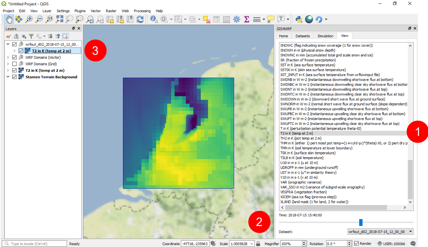
View the results

If you wish to view or analyse the data in the output files you can use tools such as GIS4WRF, wrf-python, Ncview.

The following is an example using the Visualize Output utility in GIS4WRF for wrfout_d01_2018-07-15_12_00_00. Data are displayed geo-referenced on the map canvas. You can change the variable to display (1), slice through the simulation time-steps (2), and change the color scheme by double-clicking on the layer (3) and going into Symbology.